 DuckDB Extensions
DuckDB Extension
A5 Geospatial Index
Encode lat/lng to a pentagonal cell ID and aggregate, join, or spatially filter by that ID.
On this page
Technical Overview
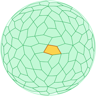
Every cell covers the same area on the globe
A5 is a pentagonal discrete global grid system, in the same family as Uber's H3 (hexagonal) and Google's S2 (square). It turns a (lon, lat) point into a single 64-bit integer cell ID that you can GROUP BY, JOIN, and index, the same way you would an H3 or S2 ID. What makes A5 different is that every cell at a given resolution covers the same area on the globe.
Why pentagons, and why equal area
A discrete global grid system chops the sphere into cells so you can drop points into buckets and count them. Those counts only mean something if the cells are about the same size wherever you look. A5 holds cell area uniform across the whole globe, and pentagons are what it uses to get there.
-
•
The problem A5 solves: When you bucket
(lon, lat)points into grid cells and compare counts, the comparison is only honest if the cells are the same size. Grids built on lat/lon rectangles or projected squares stretch badly toward the poles, so a count of 100 near the equator and 100 near a pole describe very different densities. A5 cells are equal-area at each resolution by construction, so cross-latitude density comparisons need no per-cell normalization. - • Pentagons are the cost of that uniformity: You cannot tile a sphere with regular hexagons alone — H3 pays for its hexagons with 12 unavoidable pentagon exceptions at the icosahedral vertices that traversal code must special-case. A5 instead derives its cells from a dodecahedral subdivision, giving pentagons everywhere — uniform shape, uniform area, and no exceptional cells to handle. The geometric argument is laid out on the A5 motivation page.
- • It's a thin binding over the reference library: The DuckDB functions wrap the upstream A5 Rust library, so cell IDs are identical to what the reference implementation produces — a DuckDB-computed ID round-trips through the JS/TypeScript library and back unchanged.
-
•
Sanity-check a cell before trusting it:
a5_is_valid_cellconfirms aUBIGINTis a canonically-encoded A5 cell rather than an arbitrary integer — useful right after decoding external data.a5_world_cellreturns the single root cell (ID0) that sits above all twelve resolution-0 cells and is the ultimate ancestor for anya5_cell_to_parentwalk.
How a point becomes a cell ID
Encoding a coordinate is a deterministic geometric pipeline, and the resulting 64-bit unsigned integer (UBIGINT) is self-describing — it carries its own resolution, which is why you never need a separate level column alongside it.
- • From sphere to cell: A point is located on the globe, mapped onto the face of the dodecahedron it falls in, and then placed within that face's recursive pentagonal subdivision down to the requested resolution. Resolution 0 is the small set of base cells covering the whole globe; each finer level subdivides every cell, so cell count grows by a fixed branching factor per level and resolution 30 reaches sub-square-meter precision.
-
•
Resolution is packed into the ID: The cell's position in the subdivision hierarchy and its resolution level are encoded together into the single
UBIGINT. Because the level lives inside the integer, the resolution can be recovered from a bare cell ID with no side table — and a cell at one resolution maps deterministically to its ancestor at any coarser level, which is what makes hierarchical roll-up a pure integer operation rather than a re-encode of the raw points. -
•
Pick the coarsest resolution that still separates your data: Each finer level multiplies the number of distinct cells (and therefore
GROUP BYcardinality) by the branching factor. Encode once at the finest resolution you'll ever need; roll up to coarser views in-query for free. The Cookbook and the resolution guide in the details below show the area-per-level trade-off. -
•
Cells are integers first, geometry on demand: Storage and joins use the compact integer. When you need to draw a cell,
a5_cell_to_geometrymaterializes it directly as a DuckDBGEOMETRYpolygon — the exact pattern is in the Cookbook.
Direct GEOMETRY integration
a5_cell_to_geometry, a5_cell_to_point, and a5_geometry_to_cells read and write DuckDB's built-in GEOMETRY type directly as plain little-endian WKB — no dependency on the spatial extension to produce them. Load spatial alongside A5 only when you want its functions (ST_AsGeoJSON, ST_Intersects, …) downstream of a value A5 already gave you.
-
•
Cell to geometry, and back:
a5_cell_to_geometryreturns a cell's boundary as aPOLYGON;a5_cell_to_pointreturns its center as aPOINT.a5_geometry_to_cellsruns the other direction — it accepts anyGEOMETRY(point, line, polygon, or a MULTI*/GEOMETRYCOLLECTION mix of them) and returns the covering set of A5 cells at a chosen resolution. -
•
Points snap, lines trace, polygons fill: A point geometry maps to its containing cell. A line is traced cell-by-cell along its length. A polygon is filled by cell-center containment by default — pass
overlapping := trueto additionally include cells that merely touch the polygon boundary, for genuinely gap-free coverage at the cost of some cells extending past the edge. Polygon holes are subtracted before filling. -
•
Coverings come back compacted — uncompact before you draw them: Polygon coverage from
a5_geometry_to_cellsis compacted — complete groups of sibling cells collapse to their parent — the same shapea5_compactproduces. That's the right shape for storage, transfer, and set operations, but cell boundaries at different resolutions don't nest geometrically: rendering a mixed-resolution result directly can show gaps that aren't really there. Calla5_uncompactto a single resolution first whenever you're drawing the result on a map.
A5 vs H3 vs S2
All three are global cell-based spatial indices that produce integer IDs. The shape of the cell, and how uniform its area is across the globe, is what differs — and that difference, plus ecosystem maturity, is the whole decision.
- • Cell shape: H3 tiles the world with hexagons (with 12 unavoidable pentagons at the icosahedral vertices). S2 uses curvilinear quadrilaterals derived from a cube projection. A5 uses pentagons throughout, derived from a dodecahedral subdivision — see the A5 motivation page for the geometric argument.
- • Area uniformity: H3 hex area varies by roughly a factor of 2 across the globe — not a simple latitude effect, but a smooth pattern of 20 high-area hotspots and 12 low-area ones (the icosahedron's face centers and vertices), the way the panels on a soccer ball repeat. A5 cells are equal-area at each resolution by construction, which sidesteps that pattern entirely and matters when you're computing densities or comparing counts across cells that land in different parts of it. The A5 vs H3 page in the upstream docs walks through the trade.
- • Neighbor count: Hexagons have a clean 6-neighbor structure that's nice for grid traversal. Pentagons have 5 edge-neighbors, which is slightly less convenient — but A5 has no "pentagon exceptions" the way H3 does, so neighborhood queries don't need special-case logic.
- • Ecosystem maturity: H3 is older and has a much larger ecosystem (Postgres, BigQuery, Snowflake, Spark, plus Uber's first-party libraries). S2 is widely deployed inside Google. A5 is newer — the upstream library and specification are at github.com/felixpalmer/a5. If you need the broadest tool support today, H3 is still the safest pick. Reach for A5 specifically when uniform cell area matters.
Deep Dive
Technical Details
DuckDB ↔ A5 Pentagonal Grid
A pentagon-based discrete global grid system — an alternative to H3 and S2 with equal-area cells at every resolution.
What you can do with one query
Turn a table of (longitude, latitude) points into a heatmap-style aggregation in one statement:
SELECT a5_lonlat_to_cell(longitude, latitude, 10) AS cell_id, COUNT(*) AS point_countFROM pickupsGROUP BY cell_idORDER BY point_count DESC;a5_lonlat_to_cell returns a UBIGINT you can GROUP BY, JOIN, or index — the same role H3 / S2 cell IDs play in those systems. Because A5 cells are equal-area at each resolution, the resulting counts are directly comparable across latitudes without per-cell normalization.
A5 is a newer discrete global grid system. Its specification and reference library at github.com/felixpalmer/a5 are stable, but the surrounding ecosystem is much smaller than H3’s — fewer first-party bindings (Postgres, BigQuery, Spark), fewer Stack Overflow answers, fewer existing pipelines that emit A5 IDs.
Reach for A5 specifically when uniform cell area matters: cross-latitude density comparisons, equal-area sampling, anything where H3’s hex-area variation (it swings by roughly 2× across the globe, in a smooth soccer-ball-like pattern, not just near the poles) is a problem. For “the broadest tool support” or “matching what the rest of my stack uses,” H3 is still the conservative pick. The upstream A5 vs H3 page walks through the trade in detail.
A5 vs H3 vs S2 at a glance
| Property | A5 (this extension) | H3 | S2 |
|---|---|---|---|
| Cell shape | Pentagons throughout | Hexagons (+ 12 pentagon exceptions) | Curvilinear quadrilaterals |
| Equal area | Yes, at every resolution | Approximate; varies ~2× across the globe | Approximate; varies with face |
| Edge neighbors | 5 | 6 (mostly) | 4 |
| ID type | UBIGINT |
UBIGINT |
UBIGINT |
| Resolution levels | 31 (0–30) | 16 (0–15) | 31 (0–30) |
| DuckDB extension here | Yes | Via h3 community extension |
No first-party DuckDB extension as of writing |
| Ecosystem | Newer; small but growing | Large (Uber, Postgres, BigQuery, Snowflake, …) | Large inside Google products |
If you’re already on H3 and its hex-area variation isn’t biting you, there’s no reason to switch. If you’re starting fresh and equal-area cells matter, A5 is a good pick.
Resolution guide
Pick the coarsest resolution that still distinguishes the phenomena you’re measuring — each finer level is roughly a 4× row count after GROUP BY.
| Resolution | Cell area (approx) | Typical use |
|---|---|---|
| 0–5 | 42M km² – 33k km² | Continental / country-scale rollup |
| 6–10 | 8k km² – 130 km² | Regional / metro-scale analysis |
| 11–15 | 32 km² – 32 hectares | City / district analysis |
| 16–20 | 8 hectares – 124 m² | Neighborhood / building analysis |
| 21–25 | 31 m² – 0.5 m² | Room / vehicle scale |
| 26–30 | 8 cm² – 0.03 mm² | Sub-meter precision |
a5_cell_area returns the exact equal-area size for any resolution; a5_cell_edge_length_avg returns the average edge length in meters (individual edges vary from it by roughly ±10%); a5_get_num_cells returns the global cell count.
Hierarchy and compaction
A5’s 31-level hierarchy means one encode at the finest resolution you’ll need supports every coarser zoom:
-- Encode once at the finest resolutionCREATE TABLE indexed ASSELECT *, a5_lonlat_to_cell(lon, lat, 15) AS cell_15FROM raw_points;
-- Roll up to a coarser view without re-reading raw pointsSELECT a5_cell_to_parent(cell_15, 10) AS cell_10,       COUNT(*)                       AS nFROM indexedGROUP BY cell_10;
a5_cell_to_parent walks any cell to a coarser ancestor; a5_cell_to_children goes the other way. For a region-of-interest expressed as a set of cells, a5_compact replaces complete groups of siblings with their parent — useful before storing or shipping a coverage set. a5_uncompact is the inverse.
Neighborhoods and proximity search
Three traversal primitives, depending on how you define “near”:
a5_grid_disk— all cells withinkedge-steps of a center cell.a5_grid_disk_vertex— all cells withinkvertex-steps (a slightly wider disk that includes corner-touching cells).a5_spherical_cap— all cells within a metric radius (in meters) of a center cell.
Each returns a UBIGINT[]. The typical use is to expand to a coverage set, then probe an indexed cell column with WHERE cell_id IN (UNNEST(...)) — much cheaper than ST_DWithin against raw geometries.
GEOMETRY integration
a5_cell_to_geometry and a5_cell_to_point emit DuckDB’s built-in GEOMETRY type directly — a POLYGON for the cell boundary, a POINT for its center — as plain little-endian WKB, with no dependency on the spatial extension to produce them. Load spatial alongside A5 only when you want to run its functions (ST_AsGeoJSON, ST_Intersects, ST_Area, …) against a value A5 already gave you:
INSTALL spatial; LOAD spatial;
SELECT ST_AsGeoJSON(    a5_cell_to_geometry(        a5_lonlat_to_cell(-74.0060, 40.7128, 10)    )) AS geojson;
a5_geometry_to_cells runs the other direction: it accepts any GEOMETRY (point, line, polygon, or a MULTI*/GEOMETRYCOLLECTION mix) and returns the A5 cells covering it at a chosen resolution. Points map to their containing cell, lines are traced, and polygons are filled by cell-center containment by default; pass overlapping := true to additionally include cells merely touching the boundary, for genuinely gap-free coverage. Polygon holes are subtracted before filling, and the covering set comes back compacted the same way a5_compact would.
A compacted result is the right shape for storage, transfer, and set operations — but cell boundaries at different resolutions don’t nest geometrically, so rendering a mixed-resolution result directly can show gaps that aren’t really there. Call a5_uncompact to a single resolution first whenever you draw the result on a map, as the Cookbook does.
For the raw vertex data underneath a cell’s boundary — for custom rendering pipelines that don’t go through GEOMETRY — a5_cell_to_boundary returns [lon, lat] pairs directly. The closed_ring variant repeats the first vertex at the end so the result is directly usable as a polygon ring; the segments overload interpolates additional points along each edge for smoother rendering on curved projections.
Cell validity and the world cell
a5_is_valid_cell reports whether a UBIGINT is a canonically-encoded A5 cell rather than an arbitrary integer — useful right after decoding IDs from external data. a5_world_cell returns the single root cell (ID 0) that sits above all twelve resolution-0 cells; it’s the cell 0 that a5_cell_to_boundary special-cases to an empty boundary, since the whole-globe cell has no finite polygon to draw.
Cell IDs as hex strings
A5 IDs round-trip through the canonical 16-character hex form used by the reference A5 library:
SELECT a5_u64_to_hex(a5_lonlat_to_cell(-74.0060, 40.7128, 10));-- e.g. '2607000000000000'SELECT a5_hex_to_u64('2607000000000000');-- the corresponding UBIGINTUse a5_u64_to_hex / a5_hex_to_u64 when sharing cell IDs with non-DuckDB code (the upstream JS / TypeScript library expects hex strings; integer storage is more compact inside DuckDB).
Sibling extensions
For other geospatial / spatial-key work in DuckDB:
geosilo— geographic data utilities, complementary to A5 when you need richer spatial primitives alongside cell-based indexing.lindel— space-filling curves (Hilbert, Morton). A different approach to the same “flatten 2D into a sortable 1D key” problem. Use space-filling curves when you want neighbor locality on a sorted column; use A5 when you want explicit equal-area cell membership.
Install
INSTALL a5 FROM community;
LOAD a5;
Quick Start
Encode a point as an A5 cell at resolution 10
SELECT a5_lonlat_to_cell(-74.0060, 40.7128, 10) AS nyc_cell;Aggregate point data into pentagonal buckets
SELECT a5_lonlat_to_cell(longitude, latitude, 10) AS cell_id,
       COUNT(*)                                  AS point_count
FROM   points
GROUP  BY cell_id
ORDER  BY point_count DESC;
Render a cell as a native GEOMETRY — no spatial extension needed to produce it
SELECT a5_cell_to_geometry(a5_lonlat_to_cell(-74.0060, 40.7128, 10)) AS cell_polygon;Reference
Extension Contents
Quick reference to all available functions and settings organized by category.
| Name | Type | Description |
|---|---|---|
|
Cell Properties
Inspect a specific cell — its area and average edge length in meters, its resolution level, whether it's a validly-encoded cell, and the polygon vertices that form its boundary. Useful for filtering, validation, and rendering cells on a map. |
||
| a5_cell_area() | Object type: Scalar function | Returns the area in square meters of an A5 cell at the specified resolution level |
| a5_cell_edge_length_avg() | Object type: Scalar function | Returns the average edge length in meters of an A5 cell at the specified resolution level; individual edges vary from the average by roughly +/-10% |
| a5_cell_to_boundary() | Object type: Scalar function | Returns the boundary vertices of an A5 cell as a closed ring of [lon, lat] points |
| a5_get_resolution() | Object type: Scalar function | Returns the resolution level (0-30) of an A5 cell |
| a5_is_valid_cell() | Object type: Scalar function | Returns true if the value is a valid A5 cell ID (a canonically-encoded cell). |
|
Coordinate Conversion
Translate between geographic coordinates (longitude/latitude) and A5 cell IDs in their numeric or hex string forms. Use these as your entry and exit points for indexing data into A5. |
||
| a5_cell_to_lonlat() | Object type: Scalar function | Returns the center point [longitude, latitude] of an A5 cell |
| a5_hex_to_u64() | Object type: Scalar function | Converts an A5 hex string representation to a UBIGINT cell ID |
| a5_lonlat_to_cell() | Object type: Scalar function | Converts a longitude/latitude coordinate to an A5 cell at the specified resolution |
| a5_u64_to_hex() | Object type: Scalar function | Converts a UBIGINT A5 cell ID to its hex string representation |
|
Geometry Integration
Convert cells to and from DuckDB's built-in |
||
| a5_cell_to_geometry() | Object type: Scalar function | Returns an A5 cell as a POLYGON geometry of its boundary |
| a5_cell_to_point() | Object type: Scalar function | Returns the center of an A5 cell as a POINT geometry |
| a5_geometry_to_cells() | Object type: Scalar function | Returns the A5 cells covering an arbitrary geometry at the given resolution. |
|
Hierarchy
Navigate up and down A5's 31-level resolution hierarchy. Roll cells up to a coarser parent for aggregation, expand to children for fine-grained analysis, or compact a set of sibling cells back into their parent. |
||
| a5_cell_to_children() | Object type: Scalar function | Returns the immediate child A5 cells (one resolution finer) |
| a5_cell_to_parent() | Object type: Scalar function | Returns the parent A5 cell at the specified coarser resolution |
| a5_compact() | Object type: Scalar function | Compacts a list of A5 cells by merging complete sets of sibling cells into parent cells |
| a5_get_num_children() | Object type: Scalar function | Returns the number of child cells at child_resolution that fit within a cell at parent_resolution |
| a5_uncompact() | Object type: Scalar function | Expands a compacted list of A5 cells to the specified target resolution |
|
Traversal
Find cells in a neighborhood: edge- or vertex-adjacent grid disks for fixed-step traversal, or all cells within a metric radius. Use these for proximity queries and spatial joins. |
||
| a5_grid_disk() | Object type: Scalar function | Returns all A5 cells within k edge-steps of the given cell (edge adjacency) |
| a5_grid_disk_vertex() | Object type: Scalar function | Returns all A5 cells within k vertex-steps of the given cell (vertex adjacency) |
| a5_spherical_cap() | Object type: Scalar function | Returns all A5 cells within the specified radius (in meters) of the given cell |
|
Utilities
General-purpose helpers — total cell count at a resolution, the 12 base cells covering the globe at resolution 0 (and the single root world cell above them), and parent/child cell ratios. |
||
| a5_get_num_cells() | Object type: Scalar function | Returns the total number of A5 cells at the specified resolution level (0-30) |
| a5_get_res0_cells() | Object type: Scalar function | Returns all 12 resolution 0 (root) A5 cells covering the entire globe |
| a5_world_cell() | Object type: Scalar function | Returns the A5 world cell, the root cell that covers the entire globe and is the ancestor of all resolution-0 cells |
No extension contents match that search.
API Reference
Function Reference
Practical Examples
Cookbook
Real-world recipes and patterns for common use cases.
Encode a point as a cell ID
The everyday entry point — convert (lon, lat) to a UBIGINT cell ID at a chosen resolution:
SELECT a5_lonlat_to_cell(-74.0060, 40.7128, 15) AS nyc_cell;Output
| nyc_cell |
|---|
| 2742821848331845632 |
Higher resolution = smaller cells. See a5_lonlat_to_cell for the full signature and a5_cell_area for the equal-area cell size at any resolution:
SELECT a5_cell_area(15) AS cell_area_m2;Output
| cell_area_m2 |
|---|
| 31669.04205949599 |
Aggregate point data into cells
The common heatmap pattern — bucket points by cell, then count / sum / aggregate:
SELECT a5_lonlat_to_cell(longitude, latitude, 10) AS cell_id, COUNT(*) AS point_count, AVG(amount) AS avg_amountFROM transactionsGROUP BY cell_idORDER BY point_count DESCLIMIT 100;Because A5 cells are equal-area at each resolution, the resulting counts are directly comparable across latitudes — no per-cell area normalization needed.
Recover the cell center
Round-trip a cell ID back to (lon, lat) for labeling or display:
SELECT a5_cell_to_lonlat(a5_lonlat_to_cell(-74.0060, 40.7128, 15)) AS center_coords;Output
| center_coords |
|---|
| [-74.00764805615836, 40.71280225138428] |
For a GEOMETRY point instead of a raw [lon, lat] array, use a5_cell_to_point.
Render a cell as a polygon
a5_cell_to_geometry returns the cell boundary directly as DuckDB’s built-in GEOMETRY type — no spatial extension needed to produce it. Load spatial only for functions that consume it, like ST_AsGeoJSON:
INSTALL spatial; LOAD spatial;
SELECT ST_AsGeoJSON(    a5_cell_to_geometry(        a5_lonlat_to_cell(-3.7037, 40.41677, 10)    )) AS geojson;
The cell at resolution 10 covering Madrid (-3.7037, 40.41677):
Cover a polygon (or point, or line) with cells
a5_geometry_to_cells runs the inverse of a5_cell_to_geometry — hand it any GEOMETRY and a resolution, and it returns the covering set of A5 cells. A plain ::GEOMETRY cast from WKT text works with no extension beyond a5 itself. The result comes back compacted — complete groups of sibling cells collapse to a coarser parent — the right shape for storage, transfer, and set operations. But cell boundaries at different resolutions don’t nest geometrically, so uncompact to a single resolution before drawing the cells on a map; skip that and a mixed-resolution result will show gaps that aren’t really there:
SELECT unnest(a5_uncompact( a5_geometry_to_cells( 'POLYGON((-74.02 40.70, -73.99 40.70, -73.99 40.72, -74.02 40.72, -74.02 40.70))'::GEOMETRY, 12 ), 12)) AS cell;Points map to their containing cell, lines are traced, and polygons are filled by cell-center containment by default — which really does leave a gap at the polygon’s edge, visible below where the query rectangle’s left and bottom edges cross cells whose center falls just outside it:
Pass overlapping := true for genuinely gap-free coverage — it additionally includes every cell that merely touches the boundary. Uncompact this one too before drawing it:
SELECT unnest(a5_uncompact( a5_geometry_to_cells( 'POLYGON((-74.02 40.70, -73.99 40.70, -73.99 40.72, -74.02 40.72, -74.02 40.70))'::GEOMETRY, 12, true ), 12)) AS cell;a5_geometry_to_cells’s compacted output is also the right shape to join against a uniform-resolution indexed cell column — a5_uncompact it to that resolution first — but that’s a different reason to uncompact than the rendering one above: joins care about matching resolutions, drawing cares about geometric nesting.
Roll up to a coarser resolution
Encode once at the finest resolution you’ll need, then re-aggregate at every coarser zoom without re-reading raw points:
-- Encode at resolution 15 onceCREATE TABLE indexed ASSELECT *, a5_lonlat_to_cell(lon, lat, 15) AS cell_15FROM raw_points;
-- Roll up to resolution 10SELECT a5_cell_to_parent(cell_15, 10) AS cell_10,       COUNT(*)                       AS nFROM indexedGROUP BY cell_10;
a5_get_resolution recovers the resolution from a cell ID; a5_get_num_children returns the parent/child cell ratio between two resolutions.
Drill down to children
The inverse of roll-up — get the immediate children, or all descendants at a target resolution:
-- Immediate children (one level finer)SELECT a5_cell_to_children(a5_lonlat_to_cell(-74.0060, 40.7128, 10)) AS kids;-- All descendants at resolution 12SELECT a5_cell_to_children(a5_lonlat_to_cell(-74.0060, 40.7128, 10), 12) AS descendants;Neighborhood search by cell-step
a5_grid_disk returns all cells within k edge-steps of a center cell — the typical “k-ring” pattern from H3:
SELECT unnest(a5_grid_disk(a5_lonlat_to_cell(-74.0060, 40.7128, 15), 1)) AS neighbor_cell;a5_grid_disk_vertex is the slightly wider variant that includes vertex-touching cells.
Neighborhood search by metric radius
When you have a real-world distance budget rather than a step count:
-- All cells within 5 km of Times Square at resolution 15SELECT a5_spherical_cap(a5_lonlat_to_cell(-74.0060, 40.7128, 15), 5000.0) AS nearby_cells;The typical proximity-query pattern: expand to a coverage set, then probe an indexed cell column.
WITH cells AS ( SELECT unnest(a5_spherical_cap(a5_lonlat_to_cell(-74.0060, 40.7128, 15), 5000.0)) AS c)SELECT t.*FROM transactions tJOIN cells ON cells.c = t.cell_15;Compact a coverage set
a5_compact replaces complete groups of sibling cells with their parent — fewer rows to ship, expandable on the consumer side:
SELECT a5_compact(a5_cell_to_children(a5_lonlat_to_cell(-122.4, 37.8, 5))) AS compacted;Output
| compacted |
|---|
| [1937110789722734592] |
a5_uncompact is the inverse — expand a mixed-resolution set to a uniform target resolution:
SELECT a5_uncompact([a5_lonlat_to_cell(-122.4, 37.8, 5)], 7) AS expanded;Round-trip cell IDs as hex strings
Useful when sharing cell IDs with the upstream JS / TypeScript A5 library, which uses the canonical 16-character hex form:
SELECT a5_u64_to_hex(a5_lonlat_to_cell(-122.4, 37.8, 10)) AS hex_id;-- '1ae2988000000000'SELECT a5_hex_to_u64('1ae2988000000000') AS cell_id;a5_u64_to_hex and a5_hex_to_u64 are pure conversions — store the UBIGINT form for compactness, hex for interchange.
Spatial join via shared cell ID
Encode both sides at the same resolution and join on the cell ID — much cheaper than ST_Intersects for the “are these in the same neighborhood” question:
WITH events AS ( SELECT *, a5_lonlat_to_cell(lon, lat, 12) AS cell FROM event_points),zones AS ( SELECT *, a5_lonlat_to_cell(lon, lat, 12) AS cell FROM zone_centroids)SELECT z.zone_name, COUNT(*) AS event_countFROM events eJOIN zones z USING (cell)GROUP BY z.zone_name;For polygon zones rather than centroids, encode each zone with a5_geometry_to_cells instead and UNNEST the result before joining.
Inspect the base grid
The 12 root cells covering the entire globe at resolution 0:
SELECT unnest(a5_get_res0_cells()) AS root_cell;a5_get_num_cells returns the total cell count at any resolution — useful for sizing decisions before encoding a large dataset. a5_world_cell returns the single root cell (ID 0) above all twelve of these; a5_is_valid_cell is a quick sanity check when a UBIGINT came from outside DuckDB — it rejects a cell whose encoded origin points past the 12 base cells, which is the shape of ID corruption you’d actually hit (a bit-flipped or truncated cell), not just any small integer:
SELECT a5_is_valid_cell(a5_lonlat_to_cell(-74.0060, 40.7128, 10)) AS ok, a5_is_valid_cell(63::UBIGINT << 58) AS bogus;Platform Support
Compatibility
Extension availability may vary by platform and DuckDB version. Check below to ensure this extension supports your environment before installation.
Quick Facts
Platforms
- Linux x86_64 aarch64
- Linux (musl) Not available
- macOS Intel Apple Silicon
- Windows x86_64
- WASM eh mvp threads
Compiled binary sizes
| Platform | Architecture | Size |
|---|---|---|
| Linux | x86_64 | 4.32 MB |
| Linux | aarch64 | 3.93 MB |
| macOS | Intel | 1.79 MB |
| macOS | Apple Silicon | 1.64 MB |
| Windows | x86_64 | 7.61 MB |
| WASM | eh | 180.9 KB |
| WASM | mvp | 202.3 KB |
| WASM | threads | 176.3 KB |
Compressed download size from the Haybarn extension repository.
DuckDB & Haybarn
Release calendar- DuckDB v1.5.5 Haybarn 1.5.5-rc1 Supported