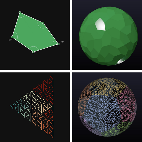
A5 Geospatial Index

Why pentagons, and why equal area

A discrete global grid system chops the sphere into cells so you can drop points into buckets and count them. Those counts only mean something if the cells are about the same size wherever you look. A5 holds cell area uniform across the whole globe, and pentagons are what it uses to get there.

• • The problem A5 solves: When you bucket (lon, lat) points into grid cells and compare counts, the comparison is only honest if the cells are the same size. Grids built on lat/lon rectangles or projected squares stretch badly toward the poles, so a count of 100 near the equator and 100 near a pole describe very different densities. A5 cells are equal-area at each resolution by construction, so cross-latitude density comparisons need no per-cell normalization.
• • Pentagons are the cost of that uniformity: You cannot tile a sphere with regular hexagons alone — H3 pays for its hexagons with 12 unavoidable pentagon exceptions at the icosahedral vertices that traversal code must special-case. A5 instead derives its cells from a dodecahedral subdivision, giving pentagons everywhere — uniform shape, uniform area, and no exceptional cells to handle. The geometric argument is laid out on the A5 motivation page.
• • It's a thin binding over the reference library: The DuckDB functions wrap the upstream A5 Rust library, so cell IDs are identical to what the reference implementation produces — a DuckDB-computed ID round-trips through the JS/TypeScript library and back unchanged.
• • Sanity-check a cell before trusting it: a5_is_valid_cell confirms a UBIGINT is a canonically-encoded A5 cell rather than an arbitrary integer — useful right after decoding external data. a5_world_cell returns the single root cell (ID 0) that sits above all twelve resolution-0 cells and is the ultimate ancestor for any a5_cell_to_parent walk.

How a point becomes a cell ID

Encoding a coordinate is a deterministic geometric pipeline, and the resulting 64-bit unsigned integer (UBIGINT) is self-describing — it carries its own resolution, which is why you never need a separate level column alongside it.

• • From sphere to cell: A point is located on the globe, mapped onto the face of the dodecahedron it falls in, and then placed within that face's recursive pentagonal subdivision down to the requested resolution. Resolution 0 is the small set of base cells covering the whole globe; each finer level subdivides every cell, so cell count grows by a fixed branching factor per level and resolution 30 reaches sub-square-meter precision.
• • Resolution is packed into the ID: The cell's position in the subdivision hierarchy and its resolution level are encoded together into the single UBIGINT. Because the level lives inside the integer, the resolution can be recovered from a bare cell ID with no side table — and a cell at one resolution maps deterministically to its ancestor at any coarser level, which is what makes hierarchical roll-up a pure integer operation rather than a re-encode of the raw points.
• • Pick the coarsest resolution that still separates your data: Each finer level multiplies the number of distinct cells (and therefore GROUP BY cardinality) by the branching factor. Encode once at the finest resolution you'll ever need; roll up to coarser views in-query for free. The Cookbook and the resolution guide in the details below show the area-per-level trade-off.
• • Cells are integers first, geometry on demand: Storage and joins use the compact integer. When you need to draw a cell, a5_cell_to_geometry materializes it directly as a DuckDB GEOMETRY polygon — the exact pattern is in the Cookbook.

Direct GEOMETRY integration

a5_cell_to_geometry, a5_cell_to_point, and a5_geometry_to_cells read and write DuckDB's built-in GEOMETRY type directly as plain little-endian WKB — no dependency on the spatial extension to produce them. Load spatial alongside A5 only when you want its functions (ST_AsGeoJSON, ST_Intersects, …) downstream of a value A5 already gave you.

• • Cell to geometry, and back: a5_cell_to_geometry returns a cell's boundary as a POLYGON; a5_cell_to_point returns its center as a POINT. a5_geometry_to_cells runs the other direction — it accepts any GEOMETRY (point, line, polygon, or a MULTI*/GEOMETRYCOLLECTION mix of them) and returns the covering set of A5 cells at a chosen resolution.
• • Points snap, lines trace, polygons fill: A point geometry maps to its containing cell. A line is traced cell-by-cell along its length. A polygon is filled by cell-center containment by default — pass overlapping := true to additionally include cells that merely touch the polygon boundary, for genuinely gap-free coverage at the cost of some cells extending past the edge. Polygon holes are subtracted before filling.
• • Coverings come back compacted — uncompact before you draw them: Polygon coverage from a5_geometry_to_cells is compacted — complete groups of sibling cells collapse to their parent — the same shape a5_compact produces. That's the right shape for storage, transfer, and set operations, but cell boundaries at different resolutions don't nest geometrically: rendering a mixed-resolution result directly can show gaps that aren't really there. Call a5_uncompact to a single resolution first whenever you're drawing the result on a map.

A5 vs H3 vs S2

All three are global cell-based spatial indices that produce integer IDs. The shape of the cell, and how uniform its area is across the globe, is what differs — and that difference, plus ecosystem maturity, is the whole decision.

• • Cell shape: H3 tiles the world with hexagons (with 12 unavoidable pentagons at the icosahedral vertices). S2 uses curvilinear quadrilaterals derived from a cube projection. A5 uses pentagons throughout, derived from a dodecahedral subdivision — see the A5 motivation page for the geometric argument.
• • Area uniformity: H3 hex area varies by roughly a factor of 2 across the globe — not a simple latitude effect, but a smooth pattern of 20 high-area hotspots and 12 low-area ones (the icosahedron's face centers and vertices), the way the panels on a soccer ball repeat. A5 cells are equal-area at each resolution by construction, which sidesteps that pattern entirely and matters when you're computing densities or comparing counts across cells that land in different parts of it. The A5 vs H3 page in the upstream docs walks through the trade.
• • Neighbor count: Hexagons have a clean 6-neighbor structure that's nice for grid traversal. Pentagons have 5 edge-neighbors, which is slightly less convenient — but A5 has no "pentagon exceptions" the way H3 does, so neighborhood queries don't need special-case logic.
• • Ecosystem maturity: H3 is older and has a much larger ecosystem (Postgres, BigQuery, Snowflake, Spark, plus Uber's first-party libraries). S2 is widely deployed inside Google. A5 is newer — the upstream library and specification are at github.com/felixpalmer/a5. If you need the broadest tool support today, H3 is still the safest pick. Reach for A5 specifically when uniform cell area matters.

Encode a point as an A5 cell at resolution 10

SELECT a5_lonlat_to_cell(-74.0060, 40.7128, 10) AS nyc_cell;

Aggregate point data into pentagonal buckets

SELECT a5_lonlat_to_cell(longitude, latitude, 10) AS cell_id,
       COUNT(*)                                  AS point_count
FROM   points
GROUP  BY cell_id
ORDER  BY point_count DESC;

Render a cell as a native GEOMETRY — no spatial extension needed to produce it

SELECT a5_cell_to_geometry(a5_lonlat_to_cell(-74.0060, 40.7128, 10)) AS cell_polygon;