Lindel computes Hilbert and Morton (Z-order) keys in DuckDB. It maps several coordinates to one integer so that sorting by the integer keeps nearby points near each other. Write a Parquet file in that order and each row group covers a compact area, so a query that filters on several columns can skip most of the file using min/max statistics.
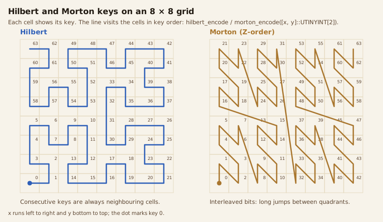
hilbert_encode and morton_encode for an 8 × 8 grid. The line follows key order.The extension was a thin wrapper around the lindel Rust crate: pass a fixed-size array, get a key back. Working on the DuckDB 2.0 build, we found that the keys didn’t sort like the values for half the types it accepted. We fixed that, then built the functions people kept writing by hand: grids for latitude and longitude, decoding by type, and box-to-range decomposition. Then we benchmarked whether the ranges help DuckDB at all. They don’t.
Negative numbers sorted after positive ones
Lindel used to encode signed integers and floats by their raw bit patterns. In two’s complement, -1 has every bit set, so it encoded as the largest possible coordinate. In IEEE 754, the sign bit is the top bit and negative magnitudes count upward from it. Sorting one-dimensional keys put the values in this order:
| Values | Previous builds | DuckDB 2.0 build |
|---|---|---|
INTEGER −2 to 2 |
0, 1, 2, −2, −1 | −2, −1, 0, 1, 2 |
DOUBLE −2 to 2 |
0, 1, 2, −1, −2 | −2, −1, 0, 1, 2 |
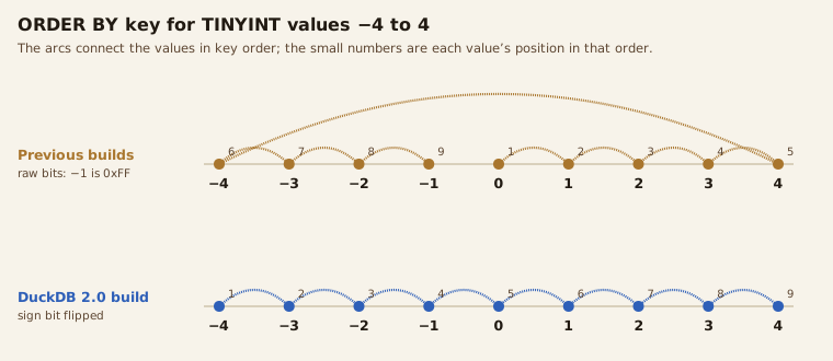
TINYINT keys from −4 to 4. With raw bits, −4 is 0xFC and −1 is 0xFF, so negative values sort after every positive one.With more dimensions, the curve kept points of the same sign together but split the space at zero. A box that crossed an axis landed in up to 2d separate parts of the curve. Nothing that relies on key order, such as decomposing a box into key ranges, could work on top of that.
The DuckDB 2.0 build maps every coordinate to order-preserving bits before encoding. Signed integers have their sign bit flipped. For floats, negative values have all bits inverted and positive values have the sign bit set, which is the standard IEEE 754 total-order trick. Dates, times, timestamps and decimals use the same mapping on their integer storage, so dates before 1970 sort first:
SELECT x, hilbert_encode([x]::INTEGER[1]) AS keyFROM (VALUES (-2), (-1), (0), (1), (2)) t(x)ORDER BY key;| x | key |
|---|---|
| −2 | 2147483646 |
| −1 | 2147483647 |
| 0 | 2147483648 |
| 1 | 2147483649 |
| 2 | 2147483650 |
Unsigned keys are unchanged. Keys computed from signed or floating-point values by earlier builds are different, so re-encode anything you’ve stored. Decoding a signed key needs return_unsigned = false, or the new typed form.
We also stopped the Rust side from panicking across the FFI boundary. An unsupported argument now returns an error to DuckDB instead of aborting the process.
Latitude, longitude and other bounded values
The documentation used to tell you to shift and scale coordinates yourself: round((lat + 90) * 1e6)::UINTEGER. Order-preserving keys make that unnecessary for correctness, but encoding DOUBLE values directly still isn’t a good layout. Two doubles make a 128-bit key whose top bits come from the exponent, so the curve runs on a roughly logarithmic scale.
hilbert_encode_bounded does the quantization properly. It scales each coordinate from a minimum to a maximum onto 2^bits cells and returns the narrowest unsigned type that holds the key. hilbert_encode_latlon is the same function with latitude and longitude bounds and 32 bits per axis, about a centimetre of resolution:
SELECT hilbert_encode_latlon(52.52, 13.405) AS berlin, hilbert_decode_latlon(hilbert_encode_latlon(52.52, 13.405)) AS decoded;| berlin | decoded |
|---|---|
| 13413847537087438956 | {'lat': 52.520000010263175, 'lon': 13.40500000398606} |
Every cell of a full grid gets a distinct key, from 0 to 2dimensions × bits − 1. The decoders return the cell centre. The bounded encoder also takes a DuckDB 2.0 GEOMETRY and encodes the centre of its bounding box. Values outside the bounds clamp to the edge cells, while hilbert_encode_latlon rejects invalid coordinates.
Grid keys nest, so a key’s parent cell k levels up is key >> (dimensions × k). We considered dedicated parent, child and neighbour functions and left them out, because a shift or a decode in SQL does the same job.
More types, a shorter call, and decoding by name
Coordinates can now be BOOLEAN, DATE, TIME, any TIMESTAMP precision, DECIMAL up to 18 digits, and ENUM, as well as integers and floats. You can pass them as separate arguments instead of building a cast array. They’re cast to their common type, and a NULL argument gives a NULL key:
SELECT hilbert_encode(pickup_date, dropoff_date) FROM trips;The original decoder needed the dimension count plus two flags, and couldn’t express a date. The new form names the type that was encoded:
SELECT hilbert_decode(hilbert_encode(DATE '2024-03-01', DATE '1965-07-04'), 'DATE[2]');-- [2024-03-01, 1965-07-04]It rejects keys too large for the type, and keys that would decode to an invalid BOOLEAN or ENUM value.
Box queries as key ranges
The feature we most expected to matter was range decomposition. Given a box, hilbert_ranges returns the sorted, disjoint key ranges that cover it:
SELECT * FROM hilbert_ranges([2, 3]::UTINYINT[2], [5, 6]::UTINYINT[2]);| lo | hi |
|---|---|
| 9 | 10 |
| 28 | 28 |
| 31 | 35 |
| 45 | 46 |
| 50 | 55 |
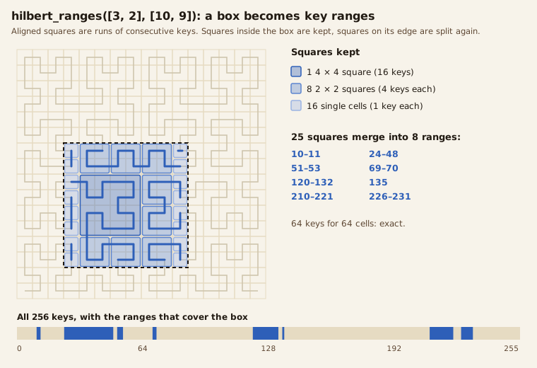
hilbert_ranges([3, 2]::UTINYINT[2], [10, 9]::UTINYINT[2]).The algorithm walks the curve’s aligned sub-squares (sub-cubes in higher dimensions), each of which is one contiguous run of keys. Squares wholly inside the box are emitted, and squares that straddle its edge are split again. The search stops after a fixed amount of work, keeps any straddling squares whole, and merges adjacent runs. If the result exceeds max_ranges (64 by default), it fills in the smallest gaps between runs. The cover can grow, but never misses a point in the box. Capped at four ranges, a box of 11,682 points on a 256 × 256 grid was covered by 13,999 keys. We checked exactness against every point of the grid for both curves, for signed, float and three-dimensional boxes, and for dates. hilbert_ranges_bounded does the same for grid keys.
The benchmark: sort by the key, filter on the coordinates
We generated 20 million uniformly random USMALLINT points and wrote them twice with 100,000-row groups: once in random order and once sorted by hilbert_encode(x, y). We also loaded both into native DuckDB tables. Then we ran a small box (1,360 matching rows) and a large one (166,920 rows) as a plain coordinate filter:
SELECT count(*) FROM 'points.parquet'WHERE x BETWEEN 30000 AND 30600 AND y BETWEEN 12000 AND 12500;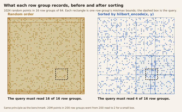
- Random order
- Hilbert-sorted
| Query | Random order | Hilbert-sorted | Row groups read |
|---|---|---|---|
| Parquet, small box | |||
| Parquet, large box | |||
| Native table, small box | |||
| Native table, large box |
AWS c6g.12xlarge, 16 threads, median of five runs in a warm session. Row groups overlapping the box from parquet_metadata().
On Parquet, sorting took both queries from 20 ms to 8 ms. The reason shows up in the file’s statistics. In random order, every one of the 200 row groups spans nearly the whole coordinate range, so none can be skipped. After sorting, the small box overlapped 2 row groups and the large box 7. DuckDB’s native tables keep the same min/max zone maps, and the sorted table answered in 2–3 ms against 6 ms.
Then we added the key ranges, joining the sorted data against hilbert_ranges with a 32-range budget and keeping the coordinate filter:
SELECT count(*) FROM 'points.parquet' p, hilbert_ranges([30000, 12000]::USMALLINT[2], [30600, 12500]::USMALLINT[2], 32) rWHERE p.k BETWEEN r.lo AND r.hi AND x BETWEEN 30000 AND 30600 AND y BETWEEN 12000 AND 12500;| Query, median of five | Small box | Large box |
|---|---|---|
| Parquet, random order, coordinate filter | 20 ms | 20 ms |
| Parquet, Hilbert-sorted, coordinate filter | 8 ms | 8 ms |
Parquet, Hilbert-sorted, join on hilbert_ranges |
9 ms | 23 ms |
| Native table, random order, coordinate filter | 6 ms | 6 ms |
| Native table, Hilbert-sorted, coordinate filter | 2 ms | 3 ms |
Native table, Hilbert-sorted, join on hilbert_ranges |
4 ms | 23 ms |
The join was never faster. On the large box it was 2.9× slower on Parquet and 7.7× slower on the native table. The coordinate filter already prunes to the same few row groups, because sorting made the row-group bounds tight. The join adds a range join that DuckDB evaluates row by row. Generating the ranges as a literal k BETWEEN … OR … predicate was slower too.
So the ranges aren’t a DuckDB query optimization, and we’ve documented them that way. They’re for systems that store or index only the key: a key-value store, an engine with a B-tree on the key column, or files partitioned by key range. In DuckDB, the advice is simpler. Sort by the key when you write the data, and filter on the original columns.
Code and measurement details
| Item | Detail |
|---|---|
| Lindel | d978907 on the v2.0 branch, extension version 2026110602 |
| DuckDB | d54cbbe, a DuckDB 2.0 development checkout |
| Machine | AWS c6g.12xlarge (48 Graviton2 cores, 96 GiB), SET threads = 16 |
| Data | 20,000,000 points, x and y uniform over USMALLINT, 100,000-row groups, 156 MB sorted and 240 MB unsorted as Parquet |
| Boxes | Small: x 30,000–30,600, y 12,000–12,500. Large: x 20,000–26,000, y 40,000–46,000 |
| Timing | DuckDB shell .timer, five runs per query in one warm session, median reported |
Row-group overlap comes from parquet_metadata(): a row group counts if its x and y min/max ranges both intersect the box. The tests cover each new function for both curves, including brute-force checks that the key ranges cover exactly the points in the box. The extension page documents every function. If something doesn’t behave as described, open an issue.