A support team lead asks a reasonable question: when a customer calls in a repair, what should we tell them about how long it will take? The repair tickets are already in DuckDB. The average is easy to compute and nearly useless. Repair times are skewed — most jobs are quick and a few drag on — so the average promises too much to the unlucky customers and too little to everyone else. The team needs the shape of the distribution, not just its center.
That is usually where the analysis leaves the database. Someone exports a column, opens a notebook, fits a few distributions with SciPy, and pastes numbers back into a dashboard. The answer drifts out of date the moment new tickets arrive.
Stochastic keeps the whole analysis in SQL. It exposes 36 probability distributions as DuckDB functions — densities, CDFs, quantiles, sampling, and moments — and its DuckDB 2.0 build adds what this question needs most: aggregates that fit a distribution to a column, say how well it fits, and test hypotheses about it. Here is the support team’s question, answered start to finish, followed by the reason you can trust the answer.
Stochastic installs from the Query Farm extension repository:
SET allow_extension_repositories = 'allowed';
CREATE EXTENSION REPOSITORY IF NOT EXISTS query_farm    WITH PREFIX 'https://duckdb-extensions.query.farm';
INSTALL stochastic FROM query_farm;LOAD stochastic FROM query_farm;
A first fit
Start with fifteen recent repair times, in hours:
CREATE TABLE repair_hours ASSELECT * FROM (VALUES (1.2), (0.7), (2.9), (1.8), (0.4), (3.6), (1.1), (2.2), (5.3), (0.9), (1.6), (2.4), (0.8), (3.1), (1.4)) t(hours);Durations like these are often modeled with a gamma distribution, so that’s a natural first guess. Fitting it is one aggregate:
SELECT round(COLUMNS(*), 3)FROM (SELECT unnest(dist_gamma_fit(hours)) FROM repair_hours);| shape | scale | log_likelihood | aic | bic |
|---|---|---|---|---|
| 2.487 | 0.788 | -22.326 | 48.652 | 50.068 |
The fit estimates the parameters by maximum likelihood: it picks the shape and scale under which the fifteen observed times are most probable. They come back as a STRUCT whose fields are named like the parameters of the other gamma functions; unnest spreads the fields into columns, and COLUMNS(*) rounds them all. Drawn over the data, the fitted density follows the cluster of quick repairs and stretches a long tail out to the 5.3-hour job:
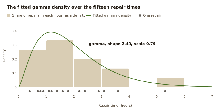
dist_gamma_pdf(2.49, 0.79, x), evaluated by the extension. The bars are the share of repairs in each hour, scaled so their area is 1 like the curve's.The last three fields are new in this release, and they say how good the fit is. log_likelihood measures how well the fit explains the data: it’s the sum, over the fifteen repairs, of the logarithm of the curve’s height at each one. The higher it is, the less surprising the data is under the fit. On its own, it can’t choose between distributions, because one with more parameters can always bend closer to the data, whether or not the extra flexibility is real.
The Akaike and Bayesian information criteria, AIC and BIC, correct for that. Both turn the log-likelihood into a cost, −2 × log-likelihood, and add a charge for each of the k fitted parameters:
- AIC = 2k − 2 × log-likelihood
- BIC = k × ln(n) − 2 × log-likelihood, where n is the number of observations
The gamma has two parameters and the sample has fifteen repairs, so its AIC is 4 + 44.65 = 48.65 and its BIC is 2 × ln(15) + 44.65 = 50.07. Lower is better for both. Neither number means anything alone; only the difference between two fits of the same data does. The two criteria differ in the charge. AIC charges 2 per parameter and favors the fit that will best predict new repairs. BIC charges ln(n), 2.7 here and more as data accumulates, so it leans harder toward simpler distributions.
Was gamma the right guess?
A first guess is only a guess. Log-normal and Weibull distributions describe durations just as often, and nothing about fifteen numbers says which is right. dist_fits fits a list of candidates to the same column in one pass and ranks them:
SELECT distribution, round(aic, 2) AS aic, round(aicc, 2) AS aicc, round(bic, 2) AS bic, round(aicc_weight, 3) AS weightFROM (SELECT unnest(dist_fits(hours, ['gamma', 'lognormal', 'weibull', 'exponential', 'normal']), recursive := true) FROM repair_hours);| distribution | aic | aicc | bic | weight |
|---|---|---|---|---|
| lognormal | 48.5 | 49.5 | 49.92 | 0.346 |
| gamma | 48.65 | 49.65 | 50.07 | 0.321 |
| weibull | 49.28 | 50.28 | 50.7 | 0.234 |
| exponential | 52.19 | 52.5 | 52.9 | 0.077 |
| normal | 53.96 | 54.96 | 55.38 | 0.023 |
Each row is the same fit the distribution’s own aggregate returns, with its parameters in a MAP and two more columns. The ranking uses AICc, the small-sample correction of AIC. AIC’s charge of 2 per parameter is fair for a large sample but too lenient for a small one, so AICc adds 2k(k + 1) / (n − k − 1). For a two-parameter fit of fifteen repairs that’s 1.0, for the one-parameter exponential 0.31, and with thousands of observations it all but vanishes. The weight column is the Akaike weight: each candidate’s share of the evidence, summing to 1 across the list.
The log-normal edges out the gamma, but by 0.15, and the weights say the same thing more plainly: 35% against 32%. A common rule of thumb treats differences under 2 as no real preference. Drawing all five fits over the same data shows why:
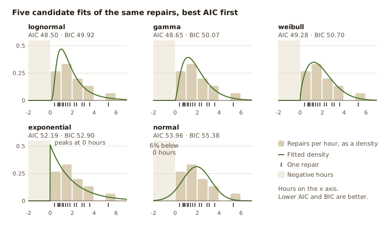
The log-normal, gamma, and Weibull curves are nearly indistinguishable where the data is, so with fifteen observations the honest conclusion is that all three are plausible. The other two are not. The normal ignores the skew and puts 6% of repairs below zero hours. The exponential is highest at zero, where no repair was that short. BIC narrows the exponential’s gap, since it has a single parameter and pays the smallest charge, but it still trails by about 3.
Those five were our candidates, though, and a short list mostly confirms what we already believed. Leave the list out and dist_fits tries every continuous fit it has. The slice keeps the top five:
SELECT distribution, cardinality(parameters) AS k, round(aicc, 2) AS aicc, round(aicc_weight, 3) AS weightFROM (SELECT unnest(dist_fits(hours)[1:5], recursive := true) FROM repair_hours);| distribution | k | aicc | weight |
|---|---|---|---|
| rayleigh | 1 | 48.78 | 0.206 |
| inverse_gaussian | 2 | 49.39 | 0.152 |
| lognormal | 2 | 49.5 | 0.143 |
| gamma | 2 | 49.65 | 0.133 |
| weibull | 2 | 50.28 | 0.097 |
The winner is one nobody suggested. The Rayleigh distribution has a single parameter, so AICc charges it the least, and its fixed shape happens to suit this sample. The inverse Gaussian, a model of the time until a drifting process first crosses a threshold, lands second. Thirteen fits are ranked in all. The beta comes last with no score and a note, “values must be between 0 and 1 (exclusive)”, because repair times aren’t proportions. A candidate that can’t be fitted says why rather than disappearing or failing the query.
But the top five are within 1.5 of each other, so the wider search hasn’t found a better model. It has found more models the data can’t rule out, and they don’t agree on the part the team cares about. The Rayleigh puts the 95th percentile at 4.05 hours. The log-normal and inverse Gaussian put it at 4.8. When the evidence can’t separate the candidates, the choice belongs to the consequences. A promise that is too short is worse than one that is too long, so the team takes the log-normal, the more cautious of the leaders, and notes that it’s a close call. A single fitted average never prompts that kind of caveat.
Stochastic has fits for 22 distributions, from the familiar normal and Poisson to the Weibull, Cauchy, inverse Gaussian, and negative binomial. dist_fits tries the continuous ones by default. It skips three: the uniform and Pareto, whose fitted bounds are just the sample’s extremes, and the standard Student’s t, which is centered at zero with unit scale and fits only its degrees of freedom. Name any of them, or the discrete candidates, to include them.
Turning the fit into an answer
The fitted parameters feed straight into the rest of the extension. What does a bad day look like, and how often will a repair take longer than the four hours the team usually quotes?
WITH fit AS (SELECT dist_lognormal_fit(hours) AS f FROM repair_hours)SELECT round(dist_lognormal_quantile(f.mean, f.stddev, 0.95), 2) AS p95_hours, round(dist_lognormal_cdf_complement(f.mean, f.stddev, 4.0), 4) AS p_over_4_hours, round(dist_lognormal_ks_test(hours, f.mean, f.stddev).p_value, 3) AS ks_p_valueFROM repair_hours, fitGROUP BY f;| p95_hours | p_over_4_hours | ks_p_value |
|---|---|---|
| 4.8 | 0.0844 | 1.0 |
One repair in twenty takes longer than 4.8 hours, and about one in twelve runs past four. That is a promise the team can make: “usually within four hours; plan for up to five.”
The last column is a Kolmogorov-Smirnov test of the fit, and its p-value of 1.0 deserves a moment’s suspicion. The test assumes the parameters were chosen before seeing the data. Here they were fitted to the same fifteen repairs, which makes the fit look better than it is. Read it as “no evidence against the log-normal”, not as proof.
The team lead’s next request is the one that usually sends analysis back to a notebook: the same numbers, per region. Fits are ordinary aggregates, so they work with GROUP BY, window frames, and DuckDB’s parallel execution. Staffing depends on how many tickets arrive, too, and a Poisson rate per region is one more query:
SELECT region, round(dist_poisson_fit(tickets).rate, 2) AS tickets_per_dayFROM (VALUES ('north', 4), ('north', 6), ('north', 5), ('north', 3), ('south', 9), ('south', 7), ('south', 11), ('south', 8)) t(region, tickets)GROUP BY regionORDER BY region;| region | tickets_per_day |
|---|---|
| north | 4.5 |
| south | 8.75 |
A pilot, and how far to trust it
A few weeks later, the team tries a new triage process on a handful of repairs. The pilot looks promising: twelve repairs, six each way, timed in minutes. Did the new process help, or did it get lucky? Welch’s t-test compares the two groups without assuming they vary equally:
SELECT round(COLUMNS(*), 5)FROM (SELECT unnest(welch_t_test(minutes, new_process)) FROM (VALUES (212.0, 0), (198.0, 0), (225.0, 0), (204.0, 0), (219.0, 0), (201.0, 0), (187.0, 1), (179.0, 1), (195.0, 1), (183.0, 1), (190.0, 1), (176.0, 1)) t(minutes, new_process));| t_statistic | degrees_of_freedom | p_value |
|---|---|---|
| 4.74753 | 8.67473 | 0.00116 |
A p-value of 0.001 is striking. But six repairs a side is a tiny sample, and pilots tend to be run by enthusiastic people on good days. Before rolling the process out, the team wants a proper trial, and a proper trial needs a size. Suppose the real improvement is more modest — half a standard deviation. How many repairs per group would a trial need to detect it reliably?
That question is about the test statistic when the null hypothesis is false, which is what the non-central distributions describe. They are among 14 distributions new in this release, alongside the arcsine, hypergeometric, inverse gamma, scaled inverse chi-squared, inverse Gaussian, Kolmogorov-Smirnov, skew normal, triangular, Dirichlet, and multinomial. The power of a two-sided t-test is a non-central t tail probability:
SELECT n_per_group, round(dist_non_central_t_cdf_complement( 2 * n_per_group - 2.0, -- degrees of freedom 0.5 * sqrt(n_per_group / 2.0), -- noncentrality for effect size 0.5 dist_students_t_quantile(2 * n_per_group - 2.0, 0.975)), 3) AS powerFROM (VALUES (20), (40), (64), (100)) t(n_per_group);| n_per_group | power |
|---|---|
| 20 | 0.338 |
| 40 | 0.598 |
| 64 | 0.801 |
| 100 | 0.94 |
Sixty-four repairs per group gives the conventional 80% chance of detecting the effect if it’s real — the same answer a power table gives, except that this query can be joined against the team’s actual ticket volumes to say how many weeks the trial will take.
Every step of the analysis — the fit, the model choice, the answer to the customer, the per-region rates, the test, and the plan for the next one — is a query. When new tickets arrive, rerunning it updates everything.
Why you can trust the numbers
An analysis like this is only as good as the functions underneath it. A statistics library is easy to get mostly right and hard to get entirely right. The formulas are well known; the edge cases are where the bugs hide. They show up at tiny probabilities, enormous parameters, and values that underflow to zero or overflow to infinity.
Our regular test suite checks the extension against SciPy: 1,401 assertions, with every fit compared against SciPy’s estimates and the Weibull against an exact solution of its likelihood equations. But with 829 functions, each taking several parameters, hand-written tests only cover the inputs someone thought to try. So before this release, we wrote a fuzzer to try the inputs nobody thinks of.
The fuzzer, which now ships in the repository as test/fuzz, calls every function with arguments chosen to break numerical code. It uses zero and negative zero, subnormal numbers, ±1e300, the largest DOUBLE, infinities, NaN, NULL, extreme BIGINTs, and empty or degenerate lists. That comes to about 218,000 calls. It treats anything other than a clean result, or an error that names the distribution, as a finding.
We expected a few odd error messages. Instead, the first run hung on 43 of its 46 parallel shards.
The largest group of hangs came from discrete quantiles. Boost.Math, which the extension builds on, finds a discrete quantile by stepping from one integer to the next. That’s fine for a Poisson distribution with a rate of 5, but a quantile near 10¹⁸ is a lot of steps. So is a probability so close to 1 that the CDF rounds to the same value across billions of integers. The loop never finishes in practice. We replaced it with a search that gallops out from the mean and then bisects on the CDF. Quantiles above 2^53, where DOUBLE can no longer represent every integer, are now an error instead of a wait.
Other hangs were retry loops. Several samplers drew a gamma variate and tried again whenever it underflowed to zero. With a tiny shape parameter it always does, so they retried forever. They now work in log space, where the value can’t underflow. The Kolmogorov-Smirnov density had a series that never terminated far in its tail, because one of its terms overflowed to NaN and the convergence check can never pass on NaN.
Then there were the wrong answers, which are worse than hangs because nothing tells you they happened. The non-central F survival function returned a negative probability at noncentrality 0. The non-central chi-squared mode was about half its true value for large noncentrality. The logistic log-CDF returned 1 for large arguments, a log-probability above zero. And Boost’s Newton iteration for the Kolmogorov-Smirnov quantile failed on perfectly ordinary inputs. That quantile now brackets the root and solves for it with the TOMS 748 algorithm.
Some numerical failures can’t be fixed. At a noncentrality of 10¹⁵, Boost’s series simply don’t converge. For those, the fix is to say so: the function raises an error that names the distribution instead of running for minutes or returning a plausible-looking wrong number.
SELECT dist_rayleigh_pdf(5e-324, 0.5);-- Invalid Input Error: rayleigh: the result is not a number for these argumentsThe release build now passes the full fuzz run, in under a minute, with no findings. A debug build with DuckDB’s internal assertions enabled reports no assertion failures.
If you used Stochastic before
The DuckDB 1.x build of Stochastic had 22 distributions; this one has 36. Most existing queries keep working. Arguments are positional, so renamed parameters, such as gamma’s shape, scale, don’t affect them.
Three behaviors did change, all in the direction of saying what’s true:
- Discrete quantiles are now the smallest integer
xwithP(X <= x) >= p, the same definition R uses. Some results move by one:dist_poisson_quantile(5, 0.3)was 3 and is now 4. - Properties that don’t exist for the given parameters, such as the mean of a Cauchy distribution, return NULL rather than an error.
- Calculations that would return NaN or an impossible probability raise an error. So do noncentralities beyond 10⁸, or 1,000 for the non-central t, where Boost’s series no longer converge in reasonable time.
The rest is quieter. dist_<name>_samples returns a list of draws, and setseed makes them reproducible even in parallel. Discrete distributions have _pmf functions, and every function is categorized in duckdb_functions(). On Linux ARM64 we also stopped promoting calculations to long double, which is emulated in software there. In our benchmark of gamma and Student’s t CDFs, that made them about 100 times faster, and results are now identical across platforms.
The Stochastic documentation has the full function reference and a cookbook organized by task. Its fit reference lists every fit’s parameters and rules. If there’s a distribution, fit, or test your own questions need, tell us.