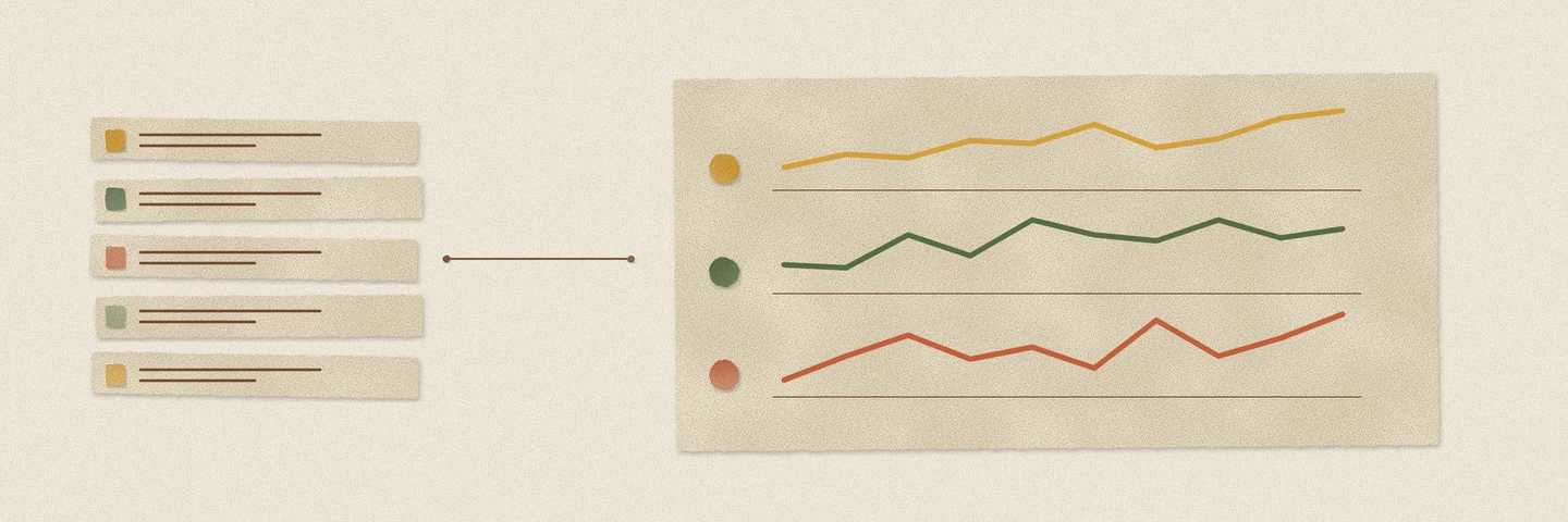
A table of averages hides the shape of a series. Two services can have the same average latency while one is steady and the other has spent the last hour getting worse. A small chart beside each row makes that difference visible without leaving the query result.
Textplot already rendered lists as sparklines. The DuckDB 2.0 build adds tp_sparkline_agg, so a group of rows can produce the chart directly. It also fixes scaling at the extremes of floating-point numbers and declares plotting options through DuckDB’s native named-parameter interface.
Plot the rows in their intended order
The aggregate takes a numeric column. Put the ordering inside the aggregate call, just as you would with list or string_agg:
CREATE TEMP TABLE readings ASSELECT * FROM (VALUES ('api', 1, 12.0), ('api', 2, 15.0),           ('api', 3, 21.0), ('api', 4, 34.0),           ('worker', 1, 31.0), ('worker', 2, 23.0),           ('worker', 3, 17.0), ('worker', 4, 13.0)) AS r(service, minute, latency_ms);
SELECT service, round(avg(latency_ms), 1) AS average_ms, tp_sparkline_agg(latency_ms, width := 12 ORDER BY minute) AS historyFROM readingsGROUP BY serviceORDER BY service;| service | average_ms | history |
|---|---|---|
| api | 20.5 | ▁▁▁▃▃▃███ |
| worker | 21.0 | ███▄▄▄▂▂▂ |
The averages are close, but the API’s latency is rising while the worker’s is falling. These are the actual strings returned by Textplot. The lowest value uses a space, so the API’s chart begins with three blank cells and the worker’s ends with three. Each chart is twelve characters wide.
An outer ORDER BY service orders the result rows. It does not order the observations within a sparkline. Without the inner ORDER BY minute, the chart follows the order in which values reach the aggregate, which is not a time-order guarantee.
The new call is equivalent to the existing form:
SELECT service, tp_sparkline(list(latency_ms ORDER BY minute), width := 12) AS historyFROM readingsGROUP BY serviceORDER BY service;This returns the same two history strings shown above. The aggregate tests compare both forms across options, groups and parallel execution. The new aggregate is a shorter expression for the same chart.
Sometimes the direction matters more than the height
The default absolute mode scales values to the sparkline’s height. For a quick view of change, use delta:
SELECT tp_sparkline_agg(v, mode := 'delta', width := 3 ORDER BY t) AS changesFROM (VALUES (1, 1.0), (2, 2.0), (3, 2.0), (4, 1.0)) AS d(t, v);| changes |
|---|
| ↑→↓ |
The series rises, stays level and falls. Themes and width use the same options as the list function. An ASCII theme is available when the destination does not render the Unicode characters well.
It also works as a window aggregate:
SELECT t, tp_sparkline_agg(v, width := 3) OVER ( ORDER BY t ROWS BETWEEN 2 PRECEDING AND CURRENT ROW ) AS recentFROM (VALUES (1, 1.0), (2, 2.0), (3, 3.0), (4, 1.0)) AS d(t, v)ORDER BY t;| t | recent |
|---|---|
| 1 | ▄▄▄ |
| 2 | █ |
| 3 | ▄█ |
| 4 | ▄█ |
Each row now carries a chart of up to three observations ending at that row. The window’s ordering supplies their sequence.
Missing values do not become zeroes
NULLs, NaNs and infinities are skipped when plotting the series. A group with no rows or only NULLs returns NULL, like other aggregates. A group containing only non-finite values returns an empty string because there is nothing finite to plot. Delta and trend modes also need at least two values.
Skipping a value closes the gap. If a missing interval has a meaning in your data, account for that before rendering; the chart does not preserve an empty time slot for it.
Each sparkline is scaled independently. Two equally tall charts can represent very different ranges, so keep an average, minimum, maximum or unit alongside them when comparing groups. The small chart tells you the shape. The numeric columns tell you its scale.
Extreme values should not flatten the chart
The plotting functions used (value - min) / (max - min) to locate values. Both endpoints can be finite while their difference overflows. For values near −1.7 × 10³⁰⁸ and +1.7 × 10³⁰⁸, that calculation could collapse everything into one bin or produce NaN before an integer conversion.
Scaling now falls back to halved values when the full range overflows. Bucket averages avoid an overflowing intermediate sum too:
SELECT '[' || tp_sparkline([-1.7e308, 1.7e308, 0.0], width := 3) || ']' AS plot;| plot |
|---|
| [ █▄] |
The zero is still halfway between the endpoints. The same scaling fix applies to bars and density plots.
Options belong in the function signature
Width, theme and other plotting options are now native named parameters. DuckDB can report their names and types in duckdb_functions(), reject unknown options when binding the query, and accept them in a different order. They remain keyword-only and must be constant expressions for the query; a column cannot choose a different width for each row.
There is one limit the compact output does not remove. The sparkline aggregate keeps the group’s finite values before rendering them. A chart that is 20 characters wide is not a constant-memory summary of an arbitrarily large group. Aggregate the observations to an appropriate interval first if you are plotting a long history.
The Textplot documentation covers the modes and themes. The new aggregate is in the DuckDB 2.0 build from the Query Farm repository.
The results shown here were produced with DuckDB 2.0.0 and Textplot build 32f0ce80ee.